Playing With Ambient

Playing With Ambient

This is a walkthrough set up by Danielle Navarro, a data scientist with some interesting generative art work. The project explores the Rayshader and ambient packages to create and render conceptual topographies on a virtual canvas, then manipulating the data to create distortions in the contours. The process utilizes a simple grid built from the ambient::long-grid function, then assigns a color set to a function that generates spatial noise with the fracture, gen_simplex, and billow functions, based on a preset seed number. This can be randomly assigned using the sample function.

The first part of generating data frames and output is fairly straightforward and provides lots of opportunities to play with various arguments in each function. The process of creating fantasy landscapes is less interesting to me, but worthwhile in the practice of exploring new functions in depth.

I’m am interested in both of these tool sets to see if they can be paired with spatial data objects to illustrate existing terrains.

Scripts From Danielle:

Set Up Canvas

# Set seed seed <- sample(1:100, 1)

# Create the intial grid

new_grid <- function(n = 1000) { ambient::long_grid( x = seq(0, 1, length.out = n), y = seq(0, 1, length.out = n) ) }

new_grid() 

# The output is a data frame with x/y coordinates

# Create spatial noise. This breaks the grid into fractals and assigns a color for each value. It is currently unclear to me how this works. 
  generate_simplex <- function(x, y, seed = NULL) {
  if(!is.null(seed)) {
    set.seed(seed)
  }
  ambient::fracture(
    noise = ambient::gen_simplex,
    fractal = ambient::billow,
    octaves = 10,
    freq_init = .02,
    frequency = ~ . * 2,
    gain_init = 1,
    gain = ~ . * .8,
    x = x,
    y = y
  )
}

It is currently unclear to me how the fracture function assigns colors to the grid, whether that is within the noise or fractal arguments. The output (shown in next section) appears as a heat map with R to Y tones.

# Create canvas. The mutate function adds a column 'paint' to the original new_grid() data frame. 

canvas <- new_grid() |> dplyr::mutate(paint = generate_simplex(x, y, seed = seed))

canvas

Create Map

# Unsure about the function or necessity of this script. The object does appear in any future scripts and removing it does not affect the output.
bitmap <- canvas |> as.array(value = paint)
bitmap[1:6, 1:6]

# This creates a plot using the as.array() function to map the values of `paint` on the new_grid dataframe. The image() function generates the output. The result is a 2d color rendering of the spatial noise generated by the generate_sinmplex function. 
canvas |>    as.array(value = paint) |>   image(axes = FALSE, asp = 1, useRaster = TRUE)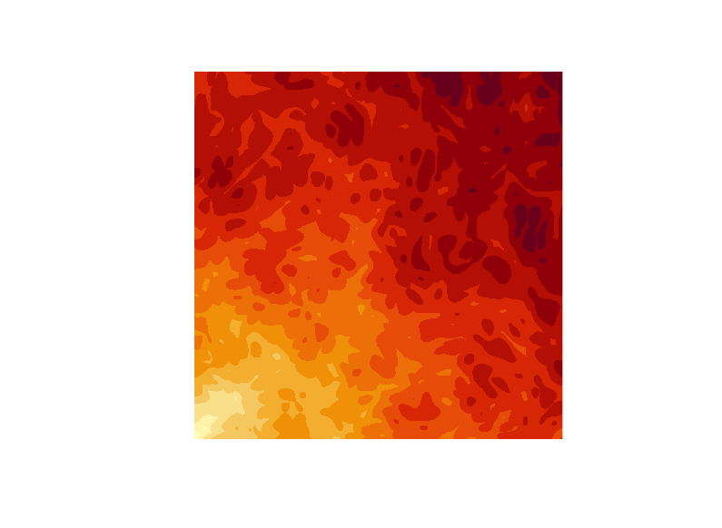 

Basic map with ambient noise function.

Render 3D

# This creates the parameters for rendering the image above in 3d. 
render <- function(mat, shades = NULL, zscale = .005) { 
  if(is.null(shades)) { 
    n <- length(unique(mat)) 
    shades <- hcl.colors(n, "YlOrRd", rev = TRUE) 
  } 
  rayshader::height_shade( 
    heightmap = mat, 
    texture = shades 
  ) 
  |> rayshader::add_shadow( 
    shadowmap = rayshader::ray_shade( 
      heightmap = mat, 
      sunaltitude = 50, 
      sunangle = 80, 
      multicore = TRUE, 
      zscale = zscale ), 
    max_darken = .2 
  ) 
  |> rayshader::plot_map() 
}

# This generates the output

canvas |> as.array(value = paint) |> render()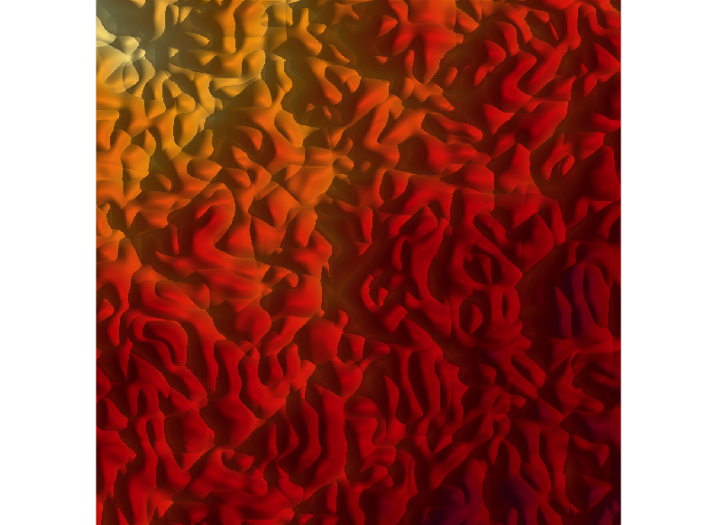

The rendered output using `Rayshader`

# sea_level creates a datum that cuts off at the median value of the 'paint' column
sea_level <- median(canvas$paint)

# The sea_level datum can be added to the canvas to create islands. This creates an 'islaands' column and sets its value to either sea_level or paint, whichever is higher. 
canvas |> 
  dplyr::mutate(
    islands = dplyr::if_else(
      condition = paint < sea_level,
      true = sea_level, 
      false = paint
    )
  ) |>
  as.array(value = islands) |>
  render()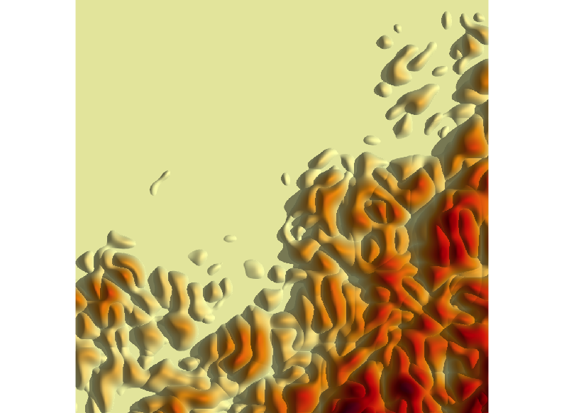

You could stop here and play with various arguments for a little while to see how each function works.

Getting Weird

This manipulates the spatial noise generator by combining the primary noise functions in ambient::fracture with ambient::gen_worley. The result feels like subducted terrain as opposed to volcanic.

generate_fancy_noise <- function(x, y, seed = NULL) { 
  if(!is.null(seed)) { 
    set.seed(seed) 
  } 
  z <- ambient::fracture(
    noise = ambient::gen_worley, 
    fractal = ambient::billow, 
    octaves = 8, freq_init = .1, 
    frequency = ~ . * 2, 
    gain_init = 3, 
    gain = ~ . * .5, 
    value = "distance2", 
    x = x, 
    y = y 
  ) 
  ambient::fracture( 
    noise = ambient::gen_simplex, 
    fractal = ambient::billow, 
    octaves = 10, 
    freq_init = .02, 
    frequency = ~ . * 2, 
    gain_init = 1, 
    gain = ~ . * .8, 
    x = x + z, 
    y = y + z 
  ) 
}

new_grid() |> dplyr::mutate( 
  height = generate_fancy_noise(x, y, seed = seed), 
  islands = dplyr::if_else( 
    condition = height < median(height), 
    true = median(height), 
    false = height 
    ) 
  ) |> as.array(value = islands) |> 
  render(zscale = .01)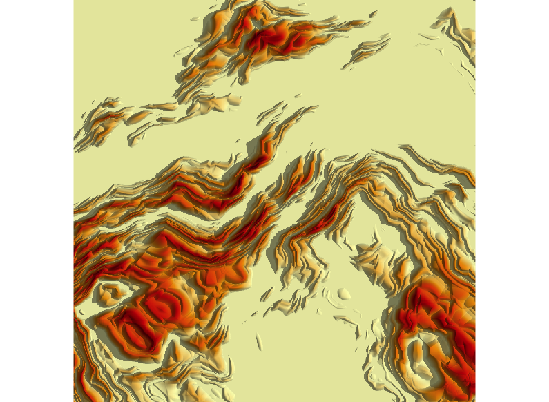 

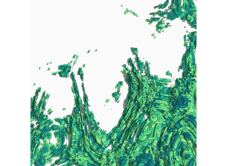
The ‘shattered’ landscape.

Additional scripts are in the project folder and utilize some interesting functions such as curl fields and curl transformations that use a discretize() function to create a terracing effect. Much of the output looks like code going through puberty, awkward and unclear as to its outcome. Additionally, there are some examples of creating different color palettes than the default YlOrRd being used by the native functions in the code. My final output looked like this:

‘Queered’ geography.

Resources

• Full text of the tutorial.
• Full script for creating islands.

References

1. Navarro, Danielle. 2023. “Shattered Landscapes.” March 13, 2023. https://blog.djnavarro.net/posts/2023-03-13_shattered-landscapes.